Note

Go to the end to download the full example code. or to run this example in your browser via Binder

Comparing Nearest Neighbors with and without Neighborhood Components Analysis#

An example comparing nearest neighbors classification with and without Neighborhood Components Analysis.

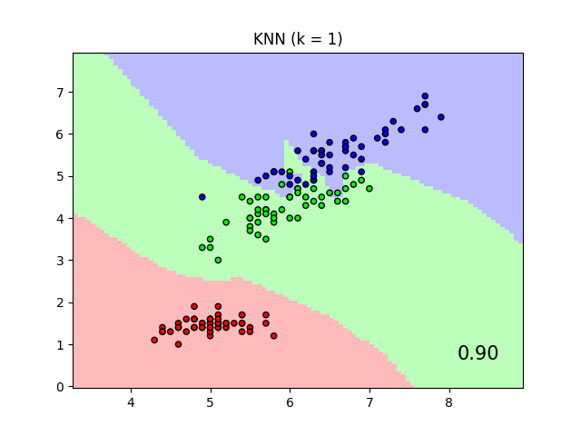
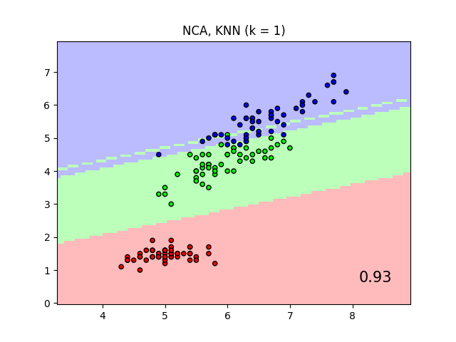
It will plot the class decision boundaries given by a Nearest Neighbors classifier when using the Euclidean distance on the original features, versus using the Euclidean distance after the transformation learned by Neighborhood Components Analysis. The latter aims to find a linear transformation that maximises the (stochastic) nearest neighbor classification accuracy on the training set.

# Authors: The scikit-learn developers
# SPDX-License-Identifier: BSD-3-Clause

import matplotlib.pyplot as plt
from matplotlib.colors import ListedColormap

from sklearn import datasets
from sklearn.inspection import DecisionBoundaryDisplay
from sklearn.model_selection import train_test_split
from sklearn.neighbors import KNeighborsClassifier, NeighborhoodComponentsAnalysis
from sklearn.pipeline import Pipeline
from sklearn.preprocessing import StandardScaler

n_neighbors = 1

dataset = datasets.load_iris()
X, y = dataset.data, dataset.target

# we only take two features. We could avoid this ugly
# slicing by using a two-dim dataset
X = X[:, [0, 2]]

X_train, X_test, y_train, y_test = train_test_split(
    X, y, stratify=y, test_size=0.7, random_state=42
)

h = 0.05  # step size in the mesh

# Create color maps
cmap_light = ListedColormap(["#FFAAAA", "#AAFFAA", "#AAAAFF"])
cmap_bold = ListedColormap(["#FF0000", "#00FF00", "#0000FF"])

names = ["KNN", "NCA, KNN"]

classifiers = [
    Pipeline(
        [
            ("scaler", StandardScaler()),
            ("knn", KNeighborsClassifier(n_neighbors=n_neighbors)),
        ]
    ),
    Pipeline(
        [
            ("scaler", StandardScaler()),
            ("nca", NeighborhoodComponentsAnalysis()),
            ("knn", KNeighborsClassifier(n_neighbors=n_neighbors)),
        ]
    ),
]

for name, clf in zip(names, classifiers):
    clf.fit(X_train, y_train)
    score = clf.score(X_test, y_test)

    _, ax = plt.subplots()
    DecisionBoundaryDisplay.from_estimator(
        clf,
        X,
        cmap=cmap_light,
        alpha=0.8,
        ax=ax,
        response_method="predict",
        plot_method="pcolormesh",
        shading="auto",
    )

    # Plot also the training and testing points
    plt.scatter(X[:, 0], X[:, 1], c=y, cmap=cmap_bold, edgecolor="k", s=20)
    plt.title("{} (k = {})".format(name, n_neighbors))
    plt.text(
        0.9,
        0.1,
        "{:.2f}".format(score),
        size=15,
        ha="center",
        va="center",
        transform=plt.gca().transAxes,
    )

plt.show()