Note
Go to the end to download the full example code. or to run this example in your browser via Binder
Categorical Feature Support in Gradient Boosting#
In this example, we compare the training times and prediction performances of
HistGradientBoostingRegressor with different encoding
strategies for categorical features. In particular, we evaluate:
“Dropped”: dropping the categorical features;
“One Hot”: using a
OneHotEncoder;“Ordinal”: using an
OrdinalEncoderand treat categories as ordered, equidistant quantities;“Native”: relying on the native category support of the
HistGradientBoostingRegressorestimator.
For such purpose we use the Ames Iowa Housing dataset, which consists of numerical and categorical features, where the target is the house sale price.
See Features in Histogram Gradient Boosting Trees for an
example showcasing some other features of
HistGradientBoostingRegressor.
See Comparing Target Encoder with Other Encoders for a comparison of encoding strategies in the presence of high cardinality categorical features.
# Authors: The scikit-learn developers
# SPDX-License-Identifier: BSD-3-Clause
Load Ames Housing dataset#
First, we load the Ames Housing data as a pandas dataframe. The features are either categorical or numerical:
from sklearn.datasets import fetch_openml

X, y = fetch_openml(data_id=42165, as_frame=True, return_X_y=True)

# Select only a subset of features of X to make the example faster to run
categorical_columns_subset = [
    "BldgType",
    "GarageFinish",
    "LotConfig",
    "Functional",
    "MasVnrType",
    "HouseStyle",
    "FireplaceQu",
    "ExterCond",
    "ExterQual",
    "PoolQC",
]

numerical_columns_subset = [
    "3SsnPorch",
    "Fireplaces",
    "BsmtHalfBath",
    "HalfBath",
    "GarageCars",
    "TotRmsAbvGrd",
    "BsmtFinSF1",
    "BsmtFinSF2",
    "GrLivArea",
    "ScreenPorch",
]

X = X[categorical_columns_subset + numerical_columns_subset]
X[categorical_columns_subset] = X[categorical_columns_subset].astype("category")

categorical_columns = X.select_dtypes(include="category").columns
n_categorical_features = len(categorical_columns)
n_numerical_features = X.select_dtypes(include="number").shape[1]

print(f"Number of samples: {X.shape[0]}")
print(f"Number of features: {X.shape[1]}")
print(f"Number of categorical features: {n_categorical_features}")
print(f"Number of numerical features: {n_numerical_features}")
Number of samples: 1460
Number of features: 20
Number of categorical features: 10
Number of numerical features: 10
Gradient boosting estimator with dropped categorical features#
As a baseline, we create an estimator where the categorical features are dropped:
from sklearn.compose import make_column_selector, make_column_transformer
from sklearn.ensemble import HistGradientBoostingRegressor
from sklearn.pipeline import make_pipeline

dropper = make_column_transformer(
    ("drop", make_column_selector(dtype_include="category")), remainder="passthrough"
)
hist_dropped = make_pipeline(dropper, HistGradientBoostingRegressor(random_state=42))
hist_dropped
Pipeline(steps=[('columntransformer',
                 ColumnTransformer(remainder='passthrough',
                                   transformers=[('drop', 'drop',
                                                  <sklearn.compose._column_transformer.make_column_selector object at 0x7fe63c9a6200>)])),
                ('histgradientboostingregressor',
                 HistGradientBoostingRegressor(random_state=42))])
In a Jupyter environment, please rerun this cell to show the HTML representation or trust the notebook. On GitHub, the HTML representation is unable to render, please try loading this page with nbviewer.org.
Parameters
| steps | [('columntransformer', ...), ('histgradientboostingregressor', ...)] | |
| transform_input | None | |
| memory | None | |
| verbose | False |
Parameters
| transformers | [('drop', ...)] | |
| remainder | 'passthrough' | |
| sparse_threshold | 0.3 | |
| n_jobs | None | |
| transformer_weights | None | |
| verbose | False | |
| verbose_feature_names_out | True | |
| force_int_remainder_cols | 'deprecated' |
<sklearn.compose._column_transformer.make_column_selector object at 0x7fe63c9a6200>
drop
passthrough
Parameters
| loss | 'squared_error' | |
| quantile | None | |
| learning_rate | 0.1 | |
| max_iter | 100 | |
| max_leaf_nodes | 31 | |
| max_depth | None | |
| min_samples_leaf | 20 | |
| l2_regularization | 0.0 | |
| max_features | 1.0 | |
| max_bins | 255 | |
| categorical_features | 'from_dtype' | |
| monotonic_cst | None | |
| interaction_cst | None | |
| warm_start | False | |
| early_stopping | 'auto' | |
| scoring | 'loss' | |
| validation_fraction | 0.1 | |
| n_iter_no_change | 10 | |
| tol | 1e-07 | |
| verbose | 0 | |
| random_state | 42 |
Gradient boosting estimator with one-hot encoding#
Next, we create a pipeline to one-hot encode the categorical features,
while letting the remaining features "passthrough" unchanged:
from sklearn.preprocessing import OneHotEncoder

one_hot_encoder = make_column_transformer(
    (
        OneHotEncoder(sparse_output=False, handle_unknown="ignore"),
        make_column_selector(dtype_include="category"),
    ),
    remainder="passthrough",
)

hist_one_hot = make_pipeline(
    one_hot_encoder, HistGradientBoostingRegressor(random_state=42)
)
hist_one_hot
Pipeline(steps=[('columntransformer',
                 ColumnTransformer(remainder='passthrough',
                                   transformers=[('onehotencoder',
                                                  OneHotEncoder(handle_unknown='ignore',
                                                                sparse_output=False),
                                                  <sklearn.compose._column_transformer.make_column_selector object at 0x7fe63c9a6500>)])),
                ('histgradientboostingregressor',
                 HistGradientBoostingRegressor(random_state=42))])
In a Jupyter environment, please rerun this cell to show the HTML representation or trust the notebook. On GitHub, the HTML representation is unable to render, please try loading this page with nbviewer.org.
Parameters
| steps | [('columntransformer', ...), ('histgradientboostingregressor', ...)] | |
| transform_input | None | |
| memory | None | |
| verbose | False |
Parameters
| transformers | [('onehotencoder', ...)] | |
| remainder | 'passthrough' | |
| sparse_threshold | 0.3 | |
| n_jobs | None | |
| transformer_weights | None | |
| verbose | False | |
| verbose_feature_names_out | True | |
| force_int_remainder_cols | 'deprecated' |
<sklearn.compose._column_transformer.make_column_selector object at 0x7fe63c9a6500>
Parameters
| categories | 'auto' | |
| drop | None | |
| sparse_output | False | |
| dtype | <class 'numpy.float64'> | |
| handle_unknown | 'ignore' | |
| min_frequency | None | |
| max_categories | None | |
| feature_name_combiner | 'concat' |
passthrough
Parameters
| loss | 'squared_error' | |
| quantile | None | |
| learning_rate | 0.1 | |
| max_iter | 100 | |
| max_leaf_nodes | 31 | |
| max_depth | None | |
| min_samples_leaf | 20 | |
| l2_regularization | 0.0 | |
| max_features | 1.0 | |
| max_bins | 255 | |
| categorical_features | 'from_dtype' | |
| monotonic_cst | None | |
| interaction_cst | None | |
| warm_start | False | |
| early_stopping | 'auto' | |
| scoring | 'loss' | |
| validation_fraction | 0.1 | |
| n_iter_no_change | 10 | |
| tol | 1e-07 | |
| verbose | 0 | |
| random_state | 42 |
Gradient boosting estimator with ordinal encoding#
Next, we create a pipeline that treats categorical features as ordered quantities, i.e. the categories are encoded as 0, 1, 2, etc., and treated as continuous features.
import numpy as np

from sklearn.preprocessing import OrdinalEncoder

ordinal_encoder = make_column_transformer(
    (
        OrdinalEncoder(handle_unknown="use_encoded_value", unknown_value=np.nan),
        make_column_selector(dtype_include="category"),
    ),
    remainder="passthrough",
)

hist_ordinal = make_pipeline(
    ordinal_encoder, HistGradientBoostingRegressor(random_state=42)
)
hist_ordinal
Pipeline(steps=[('columntransformer',
                 ColumnTransformer(remainder='passthrough',
                                   transformers=[('ordinalencoder',
                                                  OrdinalEncoder(handle_unknown='use_encoded_value',
                                                                 unknown_value=nan),
                                                  <sklearn.compose._column_transformer.make_column_selector object at 0x7fe63c9a6da0>)])),
                ('histgradientboostingregressor',
                 HistGradientBoostingRegressor(random_state=42))])
In a Jupyter environment, please rerun this cell to show the HTML representation or trust the notebook. On GitHub, the HTML representation is unable to render, please try loading this page with nbviewer.org.
Parameters
| steps | [('columntransformer', ...), ('histgradientboostingregressor', ...)] | |
| transform_input | None | |
| memory | None | |
| verbose | False |
Parameters
| transformers | [('ordinalencoder', ...)] | |
| remainder | 'passthrough' | |
| sparse_threshold | 0.3 | |
| n_jobs | None | |
| transformer_weights | None | |
| verbose | False | |
| verbose_feature_names_out | True | |
| force_int_remainder_cols | 'deprecated' |
<sklearn.compose._column_transformer.make_column_selector object at 0x7fe63c9a6da0>
Parameters
| categories | 'auto' | |
| dtype | <class 'numpy.float64'> | |
| handle_unknown | 'use_encoded_value' | |
| unknown_value | nan | |
| encoded_missing_value | nan | |
| min_frequency | None | |
| max_categories | None |
passthrough
Parameters
| loss | 'squared_error' | |
| quantile | None | |
| learning_rate | 0.1 | |
| max_iter | 100 | |
| max_leaf_nodes | 31 | |
| max_depth | None | |
| min_samples_leaf | 20 | |
| l2_regularization | 0.0 | |
| max_features | 1.0 | |
| max_bins | 255 | |
| categorical_features | 'from_dtype' | |
| monotonic_cst | None | |
| interaction_cst | None | |
| warm_start | False | |
| early_stopping | 'auto' | |
| scoring | 'loss' | |
| validation_fraction | 0.1 | |
| n_iter_no_change | 10 | |
| tol | 1e-07 | |
| verbose | 0 | |
| random_state | 42 |
Gradient boosting estimator with native categorical support#
We now create a HistGradientBoostingRegressor estimator
that can natively handle categorical features without explicit encoding. Such
functionality can be enabled by setting categorical_features="from_dtype",
which automatically detects features with categorical dtypes, or more explicitly
by categorical_features=categorical_columns_subset.
Unlike previous encoding approaches, the estimator natively deals with the categorical features. At each split, it partitions the categories of such a feature into disjoint sets using a heuristic that sorts them by their effect on the target variable, see Split finding with categorical features for details.
While ordinal encoding may work well for low-cardinality features even if categories have no natural order, reaching meaningful splits requires deeper trees as the cardinality increases. The native categorical support avoids this by directly working with unordered categories. The advantage over one-hot encoding is the omitted preprocessing and faster fit and predict time.
hist_native = HistGradientBoostingRegressor(
    random_state=42, categorical_features="from_dtype"
)
hist_native
Model comparison#
Here we use cross validation to compare the models performance in
terms of mean_absolute_percentage_error and fit times. In the
upcoming plots, error bars represent 1 standard deviation as computed across
cross-validation splits.
from sklearn.model_selection import cross_validate

common_params = {"cv": 5, "scoring": "neg_mean_absolute_percentage_error", "n_jobs": -1}

dropped_result = cross_validate(hist_dropped, X, y, **common_params)
one_hot_result = cross_validate(hist_one_hot, X, y, **common_params)
ordinal_result = cross_validate(hist_ordinal, X, y, **common_params)
native_result = cross_validate(hist_native, X, y, **common_params)
results = [
    ("Dropped", dropped_result),
    ("One Hot", one_hot_result),
    ("Ordinal", ordinal_result),
    ("Native", native_result),
]
import matplotlib.pyplot as plt
import matplotlib.ticker as ticker


def plot_performance_tradeoff(results, title):
    fig, ax = plt.subplots()
    markers = ["s", "o", "^", "x"]

    for idx, (name, result) in enumerate(results):
        test_error = -result["test_score"]
        mean_fit_time = np.mean(result["fit_time"])
        mean_score = np.mean(test_error)
        std_fit_time = np.std(result["fit_time"])
        std_score = np.std(test_error)

        ax.scatter(
            result["fit_time"],
            test_error,
            label=name,
            marker=markers[idx],
        )
        ax.scatter(
            mean_fit_time,
            mean_score,
            color="k",
            marker=markers[idx],
        )
        ax.errorbar(
            x=mean_fit_time,
            y=mean_score,
            yerr=std_score,
            c="k",
            capsize=2,
        )
        ax.errorbar(
            x=mean_fit_time,
            y=mean_score,
            xerr=std_fit_time,
            c="k",
            capsize=2,
        )

    ax.set_xscale("log")

    nticks = 7
    x0, x1 = np.log10(ax.get_xlim())
    ticks = np.logspace(x0, x1, nticks)
    ax.set_xticks(ticks)
    ax.xaxis.set_major_formatter(ticker.FormatStrFormatter("%1.1e"))
    ax.minorticks_off()

    ax.annotate(
        "  best\nmodels",
        xy=(0.05, 0.05),
        xycoords="axes fraction",
        xytext=(0.1, 0.15),
        textcoords="axes fraction",
        arrowprops=dict(arrowstyle="->", lw=1.5),
    )
    ax.set_xlabel("Time to fit (seconds)")
    ax.set_ylabel("Mean Absolute Percentage Error")
    ax.set_title(title)
    ax.legend()
    plt.show()


plot_performance_tradeoff(results, "Gradient Boosting on Ames Housing")
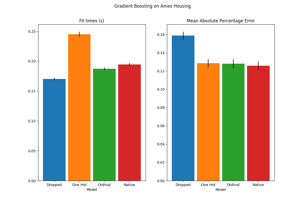
In the plot above, the “best models” are those that are closer to the down-left corner, as indicated by the arrow. Those models would indeed correspond to faster fitting and lower error.
The model using one-hot encoded data is the slowest. This is to be expected, as one-hot encoding creates an additional feature for each category value of every categorical feature, greatly increasing the number of split candidates during training. In theory, we expect the native handling of categorical features to be slightly slower than treating categories as ordered quantities (‘Ordinal’), since native handling requires sorting categories. Fitting times should however be close when the number of categories is small, and this may not always be reflected in practice.
In terms of prediction performance, dropping the categorical features leads to the worst performance. The three models that use categorical features have comparable error rates, with a slight edge for the native handling.
Limiting the number of splits#
In general, one can expect poorer predictions from one-hot-encoded data, especially when the tree depths or the number of nodes are limited: with one-hot-encoded data, one needs more split points, i.e. more depth, in order to recover an equivalent split that could be obtained in one single split point with native handling.
This is also true when categories are treated as ordinal quantities: if
categories are A..F and the best split is ACF - BDE the one-hot-encoder
model will need 3 split points (one per category in the left node), and the
ordinal non-native model will need 4 splits: 1 split to isolate A, 1 split
to isolate F, and 2 splits to isolate C from BCDE.
How strongly the models’ performances differ in practice will depend on the dataset and on the flexibility of the trees.
To see this, let us re-run the same analysis with under-fitting models where we artificially limit the total number of splits by both limiting the number of trees and the depth of each tree.
for pipe in (hist_dropped, hist_one_hot, hist_ordinal, hist_native):
    if pipe is hist_native:
        # The native model does not use a pipeline so, we can set the parameters
        # directly.
        pipe.set_params(max_depth=3, max_iter=15)
    else:
        pipe.set_params(
            histgradientboostingregressor__max_depth=3,
            histgradientboostingregressor__max_iter=15,
        )

dropped_result = cross_validate(hist_dropped, X, y, **common_params)
one_hot_result = cross_validate(hist_one_hot, X, y, **common_params)
ordinal_result = cross_validate(hist_ordinal, X, y, **common_params)
native_result = cross_validate(hist_native, X, y, **common_params)
results_underfit = [
    ("Dropped", dropped_result),
    ("One Hot", one_hot_result),
    ("Ordinal", ordinal_result),
    ("Native", native_result),
]
plot_performance_tradeoff(
    results_underfit, "Gradient Boosting on Ames Housing (few and shallow trees)"
)
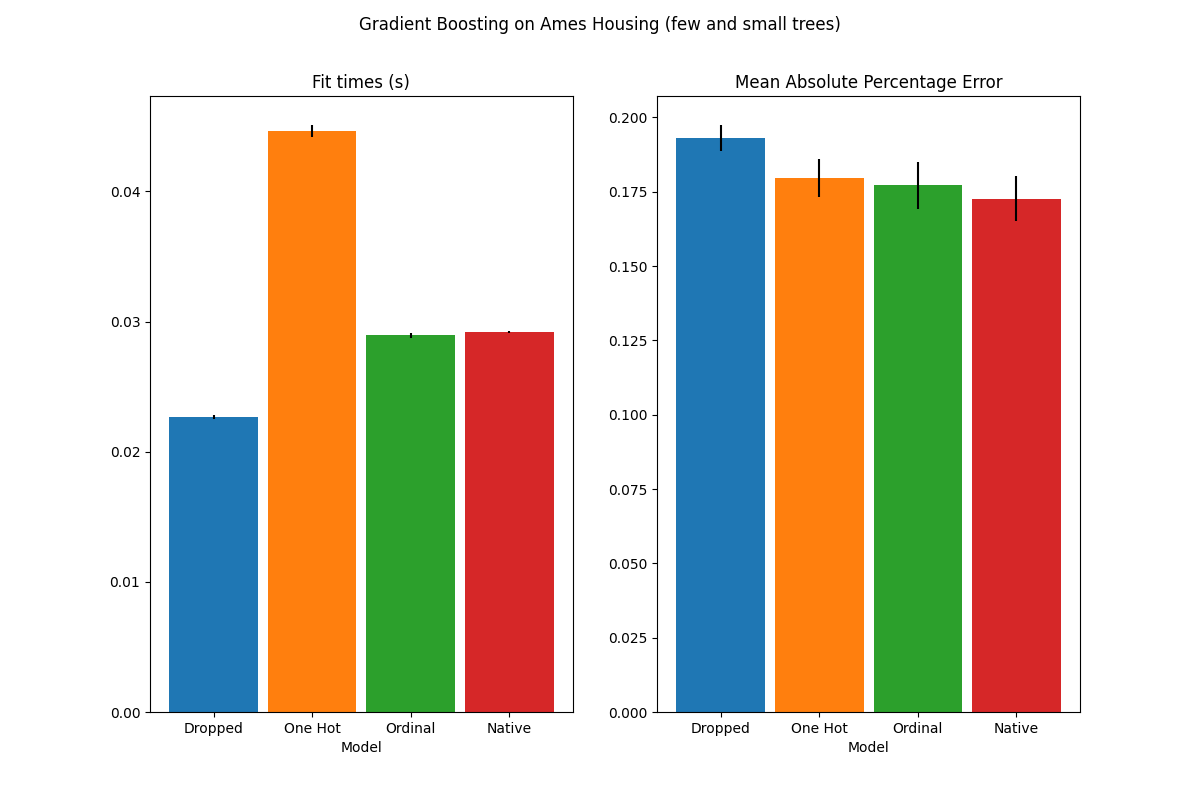
The results for these underfitting models confirm our previous intuition: the native category handling strategy performs the best when the splitting budget is constrained. The two explicit encoding strategies (one-hot and ordinal encoding) lead to slightly larger errors than the estimator’s native handling, but still perform better than the baseline model that just dropped the categorical features altogether.
Total running time of the script: (0 minutes 6.673 seconds)
Related examples